Hesaraghatta Watershed Condition Assessment Using Remote Sensing
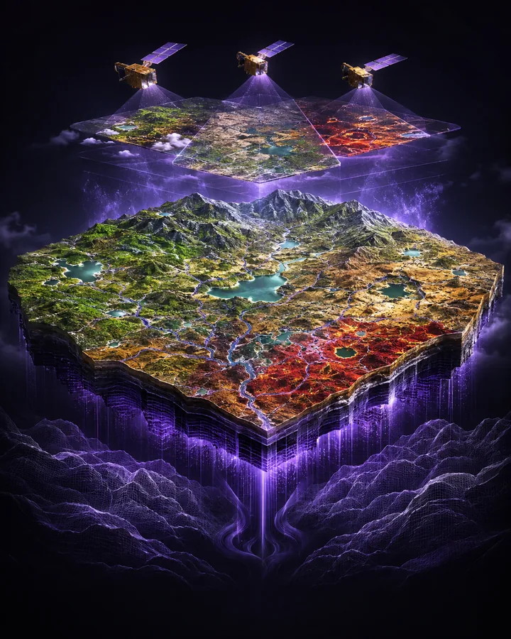
A completed civil and environmental engineering study of seasonal watershed condition across the 601 km2 Hesaraghatta watershed using three Sentinel-2 scenes, Copernicus DEM terrain and published tank-water evidence.
Project definition
Problem statement
Watershed condition changes through vegetation cycles, exposed soil, surface-water variation, drainage behaviour and land pressure, while satellite observations also change with season, cloud masking and acquisition geometry.
The engineering problem is to align a published watershed boundary, real surface-reflectance scenes and terrain data, then calculate transparent comparative evidence without calling spectral classes a field-validated land-cover map.
Project objectives
- Reproduce the published 601 km2 Hesaraghatta watershed boundary on a fixed projected grid.
- Process three cloud-screened Sentinel-2 scenes from March 2025, December 2025 and March 2026.
- Calculate NDVI, MNDWI, BSI, NDBI, transparent condition classes and a comparative screening score.
- Condition the Copernicus DEM and calculate slope, D8 flow accumulation and a declared drainage proxy.
- Separate seasonal change from a matched dry-season year comparison.
- Test the stability of the screening score under 250 plausible weight combinations per scene.
- Place current satellite results beside the published Hesaraghatta tank-water record without relabelling historical model outputs.
Project structure
Project components
Source acquisition
Retrieves the HydroShare boundary archive, exact Sentinel-2 items and Copernicus GLO-30 tile with retained source identifiers and checksums.
Raster preparation
Reprojects, clips, masks and aligns all working layers to EPSG:32643 at 60 m resolution.
Spectral analysis
Calculates four documented indices, five transparent spectral condition classes and scene summary statistics.
Terrain and drainage
Applies Priority Flood conditioning, slope calculation, acyclic D8 routing, flow accumulation and a declared drainage threshold.
Change and uncertainty
Calculates paired seasonal and dry-season changes and retains 750 seeded weight-sensitivity trials.
Historical context
Filters 225 Hesaraghatta tanks across 48 observation dates and retains the published precipitation-adjusted cluster trends.
Methodology
Project workflow
- 01Acquire sources
Download the compact HydroShare archive and stream the exact satellite and terrain assets listed in the configuration.
- 02Build the analysis grid
Union clusters 1 through 7, transform to UTM Zone 43N and reproduce the published area at 601.074 km2.
- 03Process the scenes
Apply the Sentinel-2 scene-classification mask, calculate indices and write QGIS-compatible rasters.
- 04Process terrain
Condition the DEM, calculate slope and route D8 contributing area to the drainage proxy.
- 05Compare periods
Measure seasonal and same-season changes while retaining valid paired cells and declared thresholds.
- 06Review evidence
Inspect the retained CSV, JSON, GeoJSON, GeoTIFF and labelled figures and explain every claim boundary.
Demonstration scenario
Mean NDVI rises from 0.2040 in dry March 2025 to 0.3136 after the monsoon, and moderate-vegetation signal rises from 10.04 to 58.45 percent. The comparative score rises by 8.276 points across the seasonal pair but only 0.207 points between the two dry-season scenes. The student uses the contrast to explain seasonality, uncertainty and why the score is not an official watershed rating.
Engineering
Tools and method
- Tools
- The project uses Python, Rasterio, NumPy, Pandas, SciPy, Matplotlib, QGIS, Jupyter for subject analysis, simulation, and results.
- Geospatial processing
- Rasterio, PyProj and Shapely handle projection, clipping, masking, alignment and retained raster geometry.
- Scientific calculations
- NumPy, Pandas and SciPy implement spectral equations, terrain operations, paired summaries and sensitivity experiments.
- Hydrology
- Priority Flood removes depressions and an acyclic D8 routine calculates flow accumulation without claiming surveyed channel locations.
- Visual evidence
- Matplotlib produces twenty labelled analytical figures, with two separately attributed literature figures included in the report.
- Open inspection
- GeoTIFF, GeoJSON, CSV and JSON outputs open without a custom application and the map layers can be inspected in QGIS.
- Verification
- Forty-seven tests, repository validation, accessibility checks, dependency audit and a Linux container verify the released package.
Testing
Evaluation
Evaluation measures
- Published boundary area agreement within 0.0123 percent
- Valid watershed coverage for all three satellite scenes
- Scene means for NDVI, MNDWI and the comparative score
- Five condition-class fractions and area totals per scene
- Seasonal and matched dry-season paired change statistics
- Terrain elevation, slope, flow accumulation and drainage-proxy summaries
- Fifth to ninety-fifth percentile score range from 250 weight trials per scene
- Complete source, figure, document, privacy and repository verification
Project boundaries
- The five classes are transparent spectral signals, not a field-validated land-cover classification.
- The 0 to 100 value is a comparative academic screening score and not an official watershed health rating.
- The 60 m drainage layer is a raster proxy and not a surveyed stream network or structure-siting map.
- The historical cluster trends are published precipitation-adjusted results from Penny et al. and are not recalculated field observations.
- Three scenes do not establish a long-term current trend or identify legal cause, ownership or responsibility.
- Field decisions require rainfall, streamflow, groundwater, soil, geological, water-quality and survey evidence with qualified engineering review.
Included
- 01Complete Python watershed analysis workflow
- 02Published Hesaraghatta boundary and historical tank-water evidence
- 03Three real Sentinel-2 Collection 1 Level-2A scenes
- 04Copernicus DEM elevation, slope, flow and drainage-proxy layers
- 05Seasonal and matched dry-season change analysis
- 06Seven hundred and fifty retained weight-sensitivity trials
- 07Twenty analytical figures and two licensed literature figures
- 08Forty-seven automated tests with 97.67 percent branch-aware coverage
- 09Complete project files, calculations and evidence in a private GitHub repository
- 1077-page project documentation in PDF and editable Word formats
- 1115-page setup and usage guide in PDF and editable Word formats
- 12Fifty-two annotated references
Project record
No information is collected on this page.
- Permanent project ID
- GP-CV-189WXEM
- Catalogued
- 21 Aug 2026
- Completed
- 27 Aug 2026
- Verified
- 27 Aug 2026
- Demonstration
- Included in repository
Handover
After purchase
- 01Payment is confirmed
The project is marked unavailable and cannot be purchased again.
- 02Repository access is granted
The buyer's submitted GitHub account receives access to the private repository.
- 03The purchase record is delivered
The certification sheet is prepared from the reviewed buyer details and sent privately by email.